Mar-2012 Bio435 IISER Pune[Bio435 Lab], [Bio435 Course]

---

Measuring Effective Diffusive Mobility of GFP in E. coli using Fluorescence Recovery after Photobleaching (FRAP)

Introduction

Measuring mobility and transport has been an important aspect of revealing the dynamic nature of living matter. The technique of fluorescence recovery after photobleaching (FRAP) was developed in 1976 by Axelrod et al. [1] to study the lateral transport of lipids and proteins in cell membranes. The procedure involves exposing a small region of the pool of labelled molecule to a brief intense pulse of light, thereby causing irreversible photobleaching in that region. Transport coefficients (like diffusion coefficients) can then be extracted out of the rate of recovery of fluorescence. Measurement of the signal recovery in the bleached region uses a very low intensity of light, so as to minimally photobleach the recovering signal. The choice of wavelength of photobleaching must be such that cellular components do not absorb the light to prevent photodamage to native structures (cytoplasm, organelles, DNA etc). More recently studies have begun to use the green fluorescent protein (GFP) in cells since it is a genetically encodable protein that can be complexed using standard genetic engineering methods to other proteins. Since many of the FRAP studies are conducted on (but not restricted to) proteins, this has become a useful tool. A study by Nenninger et al. [2] explored the size dependence of effective diffusion coefficients in E. coli cells using tandem GFP repeats. They could also show that for the same size of proteins as GFP, the addition of endogenous functional interactions can dramatically alter the mobility of proteins.

Depending on the nature of the experiment, sample, preparation, environment and goals of the experiment, the protocol for FRAP will need to be adapted. The illumination and experimental conditions will need to be empirically optimized for a given problem. This text provides general hints.

You will be using a confocal microscope to acquire the images as well as perform the bleaching process. It is important to understand the principle of confocal microscopy. Take a look at some of the excellent online teaching resources [3] and the standard texbook on biological confocal microscopy [4]. Please draw a basic ray-diagram for the confocal microscope when you report the data.

Principle of the Experiment

Prerequisites to FRAPinclude (taken from the EMBL EAMNET course in microscopy [5]):

a) The cells should be in a normal physiological and morphological condition as compared to cells that do not have the labelled protein.

b) The bleach rates are to be determined in fixed samples. This allows a separation of the bleach and mobility effects that might be mixed in the recovery kinetics.

To minimize photobleaching during acquisition these parameters should be adjusted:

• Image resolution can be reduced either by decreasing magnification (digitally zooming out) or reducing the pixel number of the image (e.g. 128x128 instead of 512x512)
• The time for which the laser dwell per pixel is the pixel dwell time. Using a higher scan speed will reduce mean pixel dwell time
• Using minimal laser power so the signal can be viewed but no more than necessary
• Using the appropriate fluorophores which are relatively less succeptible to photobleaching
• Frame averaging is used often in imaging to improve the quality of the image- in FRAP this is to be avoided to reduce photodamage.
• Opening the pinhole leads to increased signal with the same laser power. However it does affect the confocal sampling principle, since that depends on blocking out of focus light.

The steps in the FRAP experiment

1. A pre-bleach series (usually about 10 images) at low illumination is acquired to measure the fluorescence equilibrium before disturbance.
2. One or more spots or regions of interest (ROI) are illuminated with high intensity to disturb the fluorescence equilibrium.
3. A post-bleach image series is acquired lastly to measure the recovery kinetics of fluorescent light intensity.
4. Mobility and other parameters of the molecule of interest are extracted from this.
5. The pre-bleach series allows an estimate of the total fluorescence intensity at low intensity before bleaching is performed. This provides a reference point for fluorescence recovery- usually between 3-5 images are acquired. As a rule of the thumb, if fluorescent proteins (FP) are imaged with more than 1 image/s a prebleach series of 50-100 images is needed to reach a steady state of FPs in dark states according to Weber et al. [6].
6. Image acquisition also causes photobleaching even when done at a low light intensity. This needs to be estimated.
7. Pixel saturation is to be avoided. For an 8 bit image, the maximum intensity of 255 should be seen in minimally a few pixels. This information can be inferred from the Image Histogram (see ImageJ on how to obtain an image histogram ). The offset should be adjusted that the background pixels show gray values slightly above zero (otherwise information can be lost). To increase the dynamic range it can be advantageous to employ the 12-bit mode.

Note

In the pre- and post-bleach-series laser intensity should be attenuated to get a sufficient signal even if the images do not appear bright, to minimize photo-bleaching. In the data evaluation step the fluorescence intensity during recovery will be normalized with the pre-bleach values. In the bleaching step one or more spot(s) or region(s) of interest (ROI) are irradiated with high intensity illumination.

Ideally the bleaching event should be instantaneous, in practice it should not exceed a tenth of the half time of the recovery. Therefore for analysing rapid kinetics, more powerful lasers as well as time optimized acquisition routines are essential.

Parameters that influence the bleaching process:

1)Laser power:More laser power enables faster bleaching but also can harm the cells.

Zooming in increases the effective irradiation of the scanned area. Thus zooming in speeds up the bleaching, but the response time for switching back to the unzoomed imaging mode can delay the acquisition of the postbleach series. Which is especially undesirable when analysing rapid kinetics.

3) Scan speed:The slower the scan speed the more energy is radiated (longer pixel dwell time)

It is important to calibrate the bleached volume for each set of parameters (laser power, objective, zoom, speed, etc.), which is best done using fixed samples. A more precise definition of the bleached volume along the optical axis can be achieved using two-photon excitation.

The postbleach series monitors the dynamics and extent of the fluorescence recovery. The following hints help to improve the accuracy of the recovery detection:

1) The acquisition frequency should be adjusted to resolve the dynamic range of the recovery with good temporal resolution (rule of thumb: at least 20 data points during the time required for the half of the recovery).

2) Acquisition photobleaching should be minimized to record the recovery dynamics as precisly as possible.

3) The ideal postbleach acquisition duration is 10 to 50 times longer than the halftime (Axelrod 1976). In practice initial experiments should be conducted until no noticeable further increase in fluorescence intensity is detected.

4) When using FPs the imaging frequency should not be altered during an experiment because the fraction of FPs driven into dark states could be altered complicating the analysis of the data.

---

Evaluating the Data

Depending on the experiment there are several data evaluation steps which have to be carried out before meaningful results can be achieved:

0. Alignment of the images (only necessary if the regions of interest moved over time).

1. Fluorescence intensity quantification (obtaining the raw data)

2. Background subtraction

3. Corrections

4. Normalization

5. Mobile/immobile fraction

6. Determining t_half

---

1. Obtaining the raw data

To determine the raw FRAP data the total or average pixel values in the bleached ROI has to be determined for each timepoint. This can be done with the most confocal operating software (e.g. Zeiss LSM, Leica LCS) or with other image processing software which can handle time series (e.g. the freeware ImageJ).

2. Background subtraction

The image brightness not only originates from fluorescence of the fluorescently labelled molecules of interest. For example detector readout noise, autofluorescence (medium, glass...), and reflected light contribute to the total detected intensity. Therefore the average background value (background measurement in an area outside the cell) should be subtracted from the average pixel value in the bleaching region for each time step.

3. Corrections

Laser fluctuations, acquisition photobleaching, and fluorescence loss during photobleaching leads to intensity changes during image acquisition. In order to obtain data with a linear relationship between the measured fluorescence intensity and the concentration of fluorescent molecules, the raw data has to be corrected for these changes. One straightforward possibility to do so is to divide the background subtracted fluorescent measurement by the total cell intensity at each time point.

If this is not possible, e.g. when only a part of the cell can be imaged, alternative correction methods are available:

• Acquisition photobleaching can be corrected for by measurement of the fluorescence intensity of neighboring cells, in control experiments or the prebleach series. The fluorescence measurement at each timepoint can be divided by a function representing the acquisition photobleaching: y(n) = exp(-n/x) with n = image number can be easily determined by measuring the total fluorescence intensity of an unbleached neighboring cell or the gradual fluorescence decrease in the prebleach or postbleach images.
• Laser intensity fluctuations lang=EN-GB> can be compensated for by dividing the fluorescence measurement at each timepoint by the corresponding value of the laser monitor diode or the averaged intensity of the transmission channel outside the cell (corrected for the nonzero offset of the diode or transmission detector, respectively).

4. Normalization

To compare different experiments usually the fluorescence intensity of the average prebleach intensity is normalized to one by dividing the intensity of all timepoints by the average prebleach intensity. This can be easily done with common spreadsheet programs.

It is also possible to normalize to numbers of fluorophores by using fluorophore calibration standards (Ellenberg and Rabut).

5. Determination of the Mobile / Immobile Fraction

If the whole population of the investigated molecule is freely mobile the fluorescence intensity (background subtracted and corrected for loss of fluorescence due to the bleaching pulse) recovery curve should reach a plateau at 100% of the initial fluorescence of the prebleach. Binding of a fraction of the molecules of interest to slow or immobile structures (e.g. Nuclear envelope) reduces the recovered level of the fluorescence, the fractions can be calculated with the following equations.

Mobile fraction:

$F_M=(I_E-I_0)/(I_I-I_0)$< o:p>

Immobile fraction

F_i = 1 - F_m

With: I_E: Endvalue of the recovered fluorescence intensity

₀: first postbleach fluorescence intensity

_I: Initial (prebleach) fluorescence intensity

An additional method to measure the mobile and immobile fractions exemplified for the nucleus is described by Houtsmuller 2001 [6]. A spot in the compartment of interest is bleached over an extended period of time with relatively low laser intensity. During this extended bleaching time a large percentage of mobile molecules passes through the bleaching spot and partially will be bleached. Subsequently, the mobile molecules are allowed to completely redistribute through the nucleus (depending on their diffusion coefficient). The ratio of fluorescence intensity of confocal images before and after this procedure is then plotted against distance to the laser spot. To accurately calculate the immobile fraction from this plot one should obtain two reference curves, representing the situations in which all molecules are immobile (fixed sample) and in which all molecules are mobile (e.g. in an inducible system).

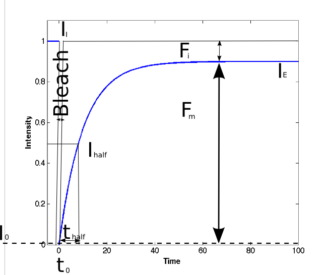
6. Determination of the halftime of the recovery (t_half)

The halftime (t_half) of recovery is the time from the bleach to the timepoint where the fluorescence intensity reaches the half (I_1/2) of the final recovered intensity (I_E). Fitting the recovery data to an exponential equation can be used to determine t_half

$y\left(t\right)=A(1-e^{^(-\tau *t)})$,

where A is the final value of the recovered intensity (I_E), t(tau)is the fitted parameter and t is the time after the bleaching pulse. After determination of t(tau) by fitting the above equation to the recovery curve the corresponding halftime of the recovery can be calculated with the following formula:

t_half = ln(0.5)/-τ

If the molecule binds to slow or immobile macromolecular structures or the diffusion is partially hindered it is very likely that the recovery curve cannot fit properly by a single exponential equation. The use of a bi-exponential equation can often overcome this problem. To compare the halftimes of a molecule under different experimental conditions (e.g. during interphase and mitosis) it is essential to use bleaching regions with the same size, relative position in the cell and scanning parameters.

Materials

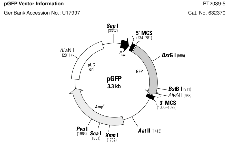
1. Escherichia coli strain K12 expressing GFP from a pGFP plasmid (Clontech, USA) are obtained. The colonies are growing in petri dishes or in small volume liquid culture with sterilized luria bertani (LB) liquid broth [make and sterilize broth 2 days before the experiment]. The expression of the pGFP plasmid that confers ampicillin resistance to the cells is controlled by lacI and is inducible with IPTG.
2. Sterile filters for sterilization of thermolabile reagents
3. Cephalexin stock solution (filter sterilized through 0.22 um filters)
4. 100 mM IPTG stock solution (filter sterilized through 0.22 um filters)
5. 100 mg/ml Ampicillin stock solution (filter sterilized through 0.22 um filters)
6. Microscopy sample holder made by sticking a coverslip to the bottom of an 8mm petri dish with a hole
7. The program ImageJ has many useful tools for extracting image intensity values. Install it on any platform- windows, Mac, Unix/Linux (its Java-based and platform independent). You will need to use the manual outline tool to identify the region from which to extract the gray values of the intensity and then store this in a text file for further data analysis using the Measure tool.
8. Data fitting can be done using MATLAB, Octave or SciPy (scientific python). You need to import the data. Perform a fit on the data of fluorescence intensity in the bleached region with the 1D diffusion equation in a finite boundary.

Protocol

(modified from Nenninger et al. 2010)

1. Cell growth and sample preparation

Bacterial cultures (2 ml) are cultivated aerobically overnight in Luria-Bertani medium supplemented with ampicillin (50 mg/ml) at 37${}^o$C under constant shaking (180 rpm). For measurements, the culture was diluted approximately 1:100 into the same media and grown at 37${}^o$C under constant shaking. Long non-septated cells are produced by adding the antibiotic cephalexin [8] to a final concentration of 30 mg/ml to a growing culture. Cells are treated with cephalexin for 90 min. In the case of slower growth, the dilution from the start culture was decreased. GFP expression was induced by adding a final concentration of IPTG in concentrations of 200 mM. Cultures were grown to the mid-exponential phase 2 hours after induction. A droplet of the culture is spotted onto Luria-Bertani agar plates and cells are allowed to settle down by drying of excess liquid. Small blocks of the agar with the cells adsorbed onto the surface were placed in a laboratory built sample holder. Since an inverted microscope is being used, the sample is placed upside down. The sample holder consists of a petridish with a hole and a coverslip stuck to the bottom to cover this hole. The holder is placed in a temperature-controlled circulating water bath. The cells were covered with a glass coverslip and placed under the microscope objective, and samples were maintained at 37${}^o$C during FRAP measurements.

FRAP measurements

The conditions described above were adapted as follows: GFP, a 50-μm confocal pinhole was used. The 100 mW argon laser with a 488 nm line is selected. The sample is imaged using a 60x oil immersion lens of numerical aperature 1.4. The intensity of the laser is reduced by a factor of 32 with neutral-density filters. The GFP fluorescence is collected in a range of 500-527 nm. Elongated cells aligned in the y-direction were selected. For photobleaching, the laser intensity is increased to maximal, the confocal pinhole is opened. Image pixel sizes were reduced to 160 by 160 pixels, with a scan speed of 9.6μs per pixel. The bleach time was reduced to approximately 0.5 s and postbleach images are recorded at 1-s intervals.

Most modern confocal microscopes have FRAP macros reduced to a single button press

FRAP data analysis

One-dimensional fluorescence profiles were extracted from images as previously described, summing data widthways across the cell using ImageJ. In order to run ImageJ install it on a windows/MAC/Linux machine- ideally in the computer lab. Using region of interests (ROI) use the measure tool to extract intensity values [9, 10]. The post-bleach profiles (It) were subtracted from the pre-bleach profile, were fitted to a Gaussian curve. Diffusion coefficients were obtained from plots of bleach depth versus time, according the one-dimensional diffusion equation:
$C=C{}_{0}R{}_0\sqrt{R{}_0^2+8\mathrm{Dt}}$

The spatial aspect of the time evolution is given by the function:
,

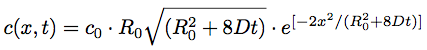where x is the 1D spatial coordinate.

.

Here t is time, C is the depth of the bleach (C₀ at t = 0), R₀ is the initial half-width (1/e²) of the bleach, and D is the lateral diffusion coefficient.

The radius of the bleach was measured from the bleaching profile extracted from the first post-bleach image (14). Presented diffusion coefficients are means obtained from measurements of at least six cells with standard deviations.

Discussion

Q1.) What diffusion coefficient do you obtain from analysing and fitting the green fluorescent protein (GFP) FRAP experimental data?

Q2.) What is the mobile fraction of GFP in E. coli in your dataset?

Q3.) What is the theoretical diffusion coefficient of the GFP molecule based on the Stoke-Einstein relation?

Q4.) What is the deviation between your measure and that of your other colleagues? Can you explain the variability? Can you add error bars? Comment on them.

Q5.) Can you think of experiments to vary expression level and consequent effect on mobility? How many copies can you estimate there might be of GFP? Justify. Is there an experimental design to measure them that you can suggest?

References

1. Nenninger, A., Mastroianni, G. & Mullineaux, C.W. Size Dependence of Protein Diffusion in the Cytoplasm of Escherichia coli. Journal of bacteriology 192, 4535-40(2010)

2. Axelrod, D. et al. Mobility measurement by analysis of fluorescence photobleaching recovery kinetics. Biophysical Journal 16, 1055-1069(1976)

3. Microscopy primer by Olympus and the Florida State University http://micro.magnet.fsu.edu/primer/index.htm

4. Pawley, J.B. Handbook of Biological Confocal Microscopy. (Springer: 2006)

5.http://www.embl.de/eamnet/

6. Weber, W. et al. Shedding light on the dark and weakly fluorescent states of green fluorescent proteins. PNAS 96, 6177-6182(1999)

7. Houtsmuller, A.B. & Vermeulen, W. Macromolecular dynamics in living cell nuclei revealed by fluorescence redistribution after photobleaching. Histochem. Cell Biol. 115, 13-21(2001)

8. Ishihara, A. et al. Coordination of flagella on filamentous cells of Escherichia coli. J. Bacteriol. 155, 228-237(1983).

9. Image J http://rsbweb.nih.gov/ij/

10. http://imagejdocu.tudor.lu/doku.php?id=plugin:analysis:frap_analysis:start